Chapter 2.5

Descriptive statistics

Proportions show the percentage of observations with a certain characteristic
Percentiles show values that relay the proportion of observations at or below the value
These values summarize data sets in different ways that can be userful in different situations
A common method of summary is to provide a value that is typical of a data set, a value which one would expect from the data set. Typically - a center

Two major types of descriptive statistics

Measures of Central Tendency
Measures of Dispersion

Mode

Definition

A natural way to typify a data set is to provide the numbers that occur frequently, to provide the modes(s)

Only one mode - data set is unimodal
Two modes - data set is bimodal
Multiple modes - data set is multimodal

In excel, use {excel}=mode.mult() to return all of the mode values
{excel}=mode() returns only one

Modes can be calculated on nominal, ordinal, interval and ratio values

Problems of mode measure

Sets like
{2, 2, 3, 3, 4, 4} ; {1, 1, 16, 17, 18} ; {1, 2, 2, 4, 5, 10, 10}
are bad to be show the central tendency

Median

Definition

A way to typify a data set is provide a value that approximately half of the values fall on each side of the value - a median

Median can be calculated on quantitative data. Qualitative is messy

Examples

{2, 2, 3, 3, 4, 4} -> 4
{1, 1, 16, 17, 18} -> 16
{1, 2, 2, 4, 5, 10, 10} -> 4

Arithmetic mean

Definition

A natural way to typify a data set is to provide a value that balances the distribution of the data set - a mean

Population mean $μ = \frac{\sum x_{i}}{N}$
Sample mean $\bar{x} = \frac{\sum x_{i}}{n}$

Mean can be calculated on quantitative data

Examples

{2, 2, 3, 3, 4, 4} -> $\bar{x} = \frac{2 + 2 + 3 + 3 + 4 + 4}{6} = 3$
{1, 1, 16, 17, 18} -> $\bar{x} = \frac{1 + 1 + 16 + 17 + 18}{5} = 4.6$
{1, 2, 2, 4, 5, 10, 10} -> $\bar{x} = \frac{1 + 2 + 2 + 4 + 5 + 10 + 10}{7} = 5$

Central Tendency and Distribution

Determine which of the three measures of central tendency is not indicated by either the pink or blue lines. Identify, with justification, which of the measures of central tendency the lines do not indicate

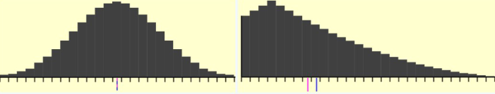
On the first graph, blue and pink indicate mean, median and mode values
On the second graph, blue indicates mean, pink indicates median
mode is not indicated

Trimmed mean

Skewed data draws the value of arithmetic mean in the direction of the skew away from the median
Extreme values that are separate from the bulk of their data, draw the value of the arithmetic mean in their direction as well
We can temper this affect by only considering a central subset of the data set

Definition -

P %

Trimmmed mean

1 Construct a central subset of data by removing the top and bottom $P$ percent of the data values
2. Compute the arithmetic mean on the central subset

Examples

1 - compute the 20% trimmed mean
a) {2, 2, 3, 3, 4, 4}
$P_{20} = 0.2 \cdot 6 = 1.2 \to 2$
{3, 3} -> $\bar{x} = \frac{3 + 3}{2} = 3$
b) {1, 1, 16, 17, 18}
$P_{20} = 0.2 \cdot 5 = 1$
{1, 16, 17} -> $\hat{x} = \frac{1 + 16 + 17}{3} = 11. (3)$
c) {1, 2, 2, 4, 5, 10, 10}
$P_{20} = 0.2 \cdot 7 = 1.4 \to 2$
{2, 4, 5} -> $\hat{x} = \frac{2 + 4 + 5}{3} = 3. (6)$
2 - construct a data set such that the 20% trimmed mean is equal to the mean
{5, 5, 5, 5, 5}
3 - construct a data set such that the 10% trimmed mean is equal to the mean
{5, 5, 5, 5, 5}
4 - construct a data set of size 6 containing multiple values so that the mean, median, and mode are all equal to 10