7 - Hypothesis Testing

Hypothesis Testing

Introduction

Definitions

Hypothesis - a claim about reality
Competing Hypothesis - a pair of opposing hypotheses regarding a particular aspect, such that one of them must be true
Null Hypothesis $H_{0}$ - Hypothesis that is acted upon as if true by default
Alternative Hypothesis $H_{1}$ - Hypothesis not presumed to be true in our actions

Poses the greater negative impact if acting as if it is true when it is indeed false
In scientific inquiry, it is typically the desired result
Hypotheses Testing - Process of collecting and weighing evidence against $H_{0}$ to determine if there is enough evidence to reject $H_{0}$ as true

Conclusions

If there is enough evidence against the $H_{0}$ then it is rejected
We reject the null hypothesis in favour of the alternative one
This does NOT prove $H_{0}$ false. This does NOT prove $H_{1}$ true
There is sufficient evidence to begin acting in accord with the alternative hypothesis
If there is not enough evidence against the $H_{0}$ , then it is not rejected
We fail to reject the null hypothesis
This does NOT prove $H_{0}$ true, nor $H_{1}$ false
There is not a strong enough reaso to alter our default position in determining how to act away from $H_{0}$

Practical judgment is necessary when determining how to act in accord with a hypothesis and the evidence

Consequences of Hypothesis Testing and Assessing Evidence

Errors

Type I Error - Rejecting a true null hypothesis
Type II Error - Failing to reject a false null hypothesis

Determining Sufficient Evidence

Given a true null hypothesis

how ofter are we okay making a type I error?
for what proportions of samples are we okay rejecting the truth because the statistics produced are rare enough?

Assessing Evidence

The p-value is the probability of obtaining evidence at least as rare as the evidence collected under the assumption that the null hypothesis is true
If the p-value is very small, it indicates that something rare or unusual happened in the case that the null hypothesis is true
If the p-value is not very small, it indicates that something routine or usual happened in the case that the null hypothesis is true
If the p-value is small enough, it makes us question whether assuming the null hypothesis is true is the right way to act
For single-tail tests, there are infinitely many parameter values in the null hypothesis. The border value is chosen for the calculation as it provides the worst-case probability value

Determining Sufficiency of Evidence

We set the standard for sufficient evidence by determining which p-values are small enough to reject the null hypothesis
If the p-value is less than the value we set, we reject the null hypothesis
We call this value the $α$ -value or significance level of the test

p-value $< α$ - reject the null hypothesis
p-value $\geq α$ - fail to reject the null hypothesis
It is possible that the collected evidence is rare enough to result in p-value under $α$ despide null hypothesis being true
The significance level is the probability of making a type I error given that the null hypothesis is true

Hypothesis Testing Procesure

Identify competing hypotheses
Set significance level $α$
Determine sample size $n$
p-value distribution is a probability calculating from the sampling distribution. Select sample size large enough so that the shape of the sampling distribution can be approximated
Select a sample via SRS
Collect and study the sample. Compute sample statistics
Compute the p-value and make statistical conclusion
p-value $< α$ - reject $H_{0}$ in favor of $H_{1}$
p-value $\geq α$ - fail to reject $H_{0}$
In light of statistics conclusion, determine if a change in behaviour is prudent and practical

Claims on Means

Hypothesis Tests on Means

$\begin{aligned} {\begin{cases} H_{0} : μ \leq μ_{0} \\ H_{1} : μ > μ_{0} \end{cases} & {\begin{cases} H_{0} : μ \geq μ_{0} \\ H_{1} : μ < μ_{0} \end{cases} & {\begin{cases} H_{0} : μ = μ_{0} \\ H_{1} : μ \neq μ_{0} \end{cases} \end{aligned}$

Each member of the population has a numerical value associated with it. We are interested in the average of these values
Need $n > 30$ (SDSM $\approx$ normal) or population normally distributed
Need a SRS

Computing the p-value

The sample statistic that we compute from our collected sample is our evidence. The value reisdes along the horizontal axis of the sampling distribution
p-value is computed by computing probability that at least as extreme as our test statistic is achieved under the assumption that the null hypothesis is true in the worst case scenario (equal to border value)
If we know the standard deviation of the sampling distribution, we can calculate the p-value easily
If we do not know the standard deviation of the sampling distribution, we must transform our problem
Many people like to transform the problem regardless of whether we know the standard deviation of the sampling distribution

The sampling distribution is approximately normal
If $σ$ is known, we transform the problem using z-score, transforming sample evidence into a test statistic z

z = \frac{\bar{x} - μ_{0}}{\frac{σ}{\sqrt{n}}} $ $ w h i c h r e s i d e s i n t h e z - d i s t r i b u t i o n I f $ σ $ i s u n k n o w n, w e t r a n s f o r m t h e p r o b l e m u s i n g t h e t - s c o r e, t r a n s f o r m i n g o u r s a m p l e e v i d e n c e i n t o a * t e s t s t a t i s t i c t * $ $ t = \frac{\bar{x} - μ_{0}}{\frac{s}{\sqrt{n}}}

which resides in the t-distribution

Excercises

Hypothesis Test
A software designer is testing the efficiency of the new version of program. He hopes that new version is faster than the last one. Both versions are run 14 times (different computers, same set of websites). Test developer's claim at the 0.01 level of significance assuming that the differences come from a normal distribution.

Old	New
12.4	10.2
13	7.8
14.5	9.3
13.2	14
10	7
16	16
14.3	16.6
9.3	5.6
14.2	15.7
9.3	7.1
11.5	7.8
13.6	6.1
9.2	4
12.4	13.2

Hypothesis tests

For the program to be faster:

\begin{array}{r} H_{0} : μ_{d} \leq 0 \\ H_{1} : μ_{d} > 0 \end{array}

We calculate all differences as: $o l d - n e w$ . If the average is positive, then the program is faster
$α = 0.01$
$n = 14$
approx, random, norm
t-test
${\bar{x}}_{d} = 2.32$
$s_{d} = 2.997$

t = \frac{{\bar{x}}_{d} - μ_{0}}{\frac{s_{d}}{\sqrt{n}}} = \frac{2.32 - 0}{\frac{2.997}{\sqrt{14}}} = 2.898

this $t$ value is is number of deviations we have to move away from 0

We put $μ_{0} = 0$ , because our question is 'is faster than', and we operate on differences, so anything $> 0$ means it's faster.

p-value: $p = 1 - t.dist (2.898, 13, 1) = 0.006$
$p-value < α$ - so we reject the null

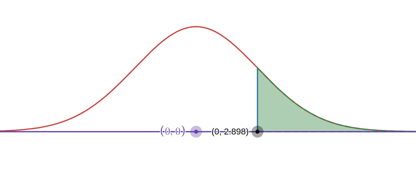
green area is the p-value, which is the area for which $t_{i} \geq t$ so the $H_{0}$ fails for (program being slower), so we reject it and accept $H_{1}$ - program being faster
The area on the left of $2.898$ border is probability that the program is faster than the old version

Claims on Proportions

Hypothesis Tests on Proportions

$\begin{aligned} {\begin{cases} H_{0} : p \leq p_{0} \\ H_{1} : p > p_{0} \end{cases} & {\begin{cases} H_{0} : p \geq p_{0} \\ H_{1} : p < p_{0} \end{cases} & {\begin{cases} H_{0} : p = p_{0} \\ H_{1} : p \neq p_{0} \end{cases} \end{aligned}$

We are interested in the percentage of members with a particular quality
We need $n p_{0} > 5$ and $n q_{0} > 5$ (SDSP $\approx$ normal) and SRS

Z-Distribution

$z = \frac{\hat{p} - p_{0}}{\sqrt{\frac{p_{0} q_{0}}{n}}} $ $ w h i c h r e s i d e s i n t h e z - d i s t r i b u t i o n$

Exercises

Harper's Index reported that 80% of all supermarket prices and in the digits of 9 or 5. From your recollection, this estimate seems too high. You randomly select 115 items from supermarket price catalogs and find that 88 have prices that end with a 9 or 5. Test the claim at the 1% level of significance.

\begin{array}{r} H_{0} : p \geq 80 % \\ H_{1} : p < 80 % \end{array}

$α = 0.01$
random
$n = 115$
$p_{0} = 0.8$
$n p_{0} > 5$ and $n q > 5$ so normal
88% have 5 or 9 at the end, so $\hat{p} = \frac{88}{115} \approx 0.75$
Doing distribution:

$μ_{\hat{p}} = 0.8$
$σ_{\hat{p}} = \sqrt{\frac{0.8 \cdot 0.2}{115}} = 0.037$
$p-value (green area) = norm.dist (\frac{88}{115}, 0.8, 0.037, 1) = 0.176$

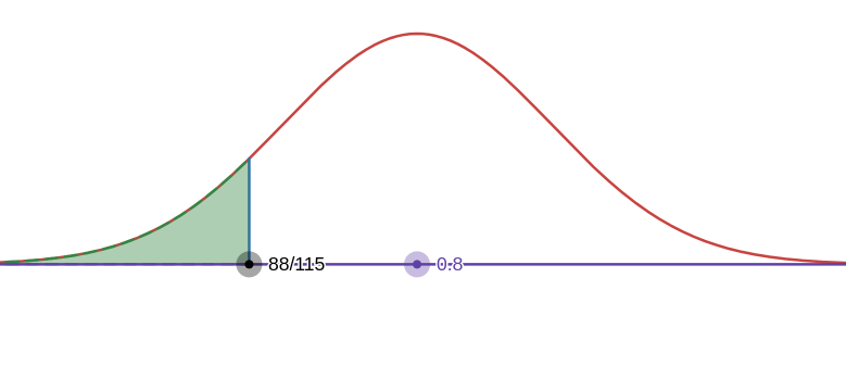
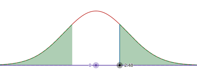
p-value is bigger than our $α$ , so we fail to reject the hypothesis $H_{0}$

Myers-Briggs estimates that about 82% of college student government leaders are extroverted. A random sample of 73 student government leaders were given the Myers-Briggs personality test; 68 of them were found to be extroverted. Test the claim that the actual percentage is different that what was reported at a significance level of 2%

\begin{array}{r} H_{0} : p = 0.82 \\ H_{1} : p \neq 0.82 \end{array}

$α = 0.02$
$n = 73$ , $p_{0} = 0.82$
it is random
$n p_{0} > 5$ and $n q_{0} > 5$ so it is normal
$\hat{p} = \frac{68}{73} = 0.93$
Doing test statistic:
$z = \frac{\hat{p} - p}{σ_{\hat{p}}} = \frac{\hat{p} - p_{0}}{\sqrt{\frac{p_{0} q_{0}}{n}}} = \frac{0.93 - 0.82}{\sqrt{\frac{0.82 \cdot 0.18}{72}}} = 2.48$

$p-value = norm.s.dist (- 2.48, 1) \cdot 2 = 0.013$
$p-value < α$ so we can reject the null

According to the Pew Research Center, the average number of FB friends is 338. A random sample of 100 users had an average of 287 friends with a standard deviation of 50 friends. Test the claim that the average number of friends is less than reported by Pew using a significance level of your choosing.

\begin{array}{r} H_{0} : μ \geq 338 \\ H_{1} : μ < 338 \end{array}

$α = 0.05$ , $n = 100$ , $\bar{x} = 287$ , $s = 50$

A delivery service claims to deliver packages from NYC to LA in 24 hours on average. It is well-agreed upon the delivery services have a standard deviation of 2 hours. Several complaints about this particular service have been made about delivery taking longer than advertised. An independent consumer agency conducted a study. A random sample of 35 packages produces a mean of 24.85 hours. Test the claim at $α = 0.04$

\begin{array}{r} H_{0} : μ = 24.0 \\ H_{1} : μ \neq 24.0 \end{array}

$n = 35$ , $\bar{x} = 24.85$ , $α = 0.04$
$z = \frac{\bar{x} - μ}{\frac{σ}{\sqrt{n}}} = \frac{24.85 - 24}{\frac{2}{\sqrt{35}}} = 2.51$
$p-value = 2 \cdot norm.s.dist (- 2.51, 1) = 0.012$
$p-value < α$ so we reject the $H_{0}$